Signal Analysis
What is Signal Analysis
Signal analysis is the process of investigating and evaluating trading signals to assess their effectiveness. It helps traders understand the strengths and weaknesses of their buying and selling signals by highlighting the relationships between a target and a signal.
By leveraging insights from signal analysis, you can:
Refine your signals for better accuracy.
Adjust backtest configurations, such as pyramiding, stop-loss settings, and other parameters.
Optimize your strategy for improved performance.
You can access to our Signal Analysis tool in the following path:
In this tutorial, we will use Signal Analysis to evaluate the effectiveness of RSI and Stochastic in identifying optimal buying and selling points.
To follow this tutorial, you need to create a market dataset that includes OHLCV, RSI, and Stochastic data of 15-minute timeframe for Apple and Microsoft from 2021/01/01 to 2021/12/30.
If you are unfamiliar with creating a market dataset or adding technical indicators, please refer to the first tutorial in the Beginner Series for detailed instructions.
RSI Signals
RSI (Relative Strength Index) is a widely used oscillator that fluctuates between 0 and 100.
When RSI > 70, it enters the overbought region, signaling a potential sell opportunity.
When RSI < 30, it enters the oversold region, signaling a potential buy opportunity.
To create buying and selling signals using RSI:
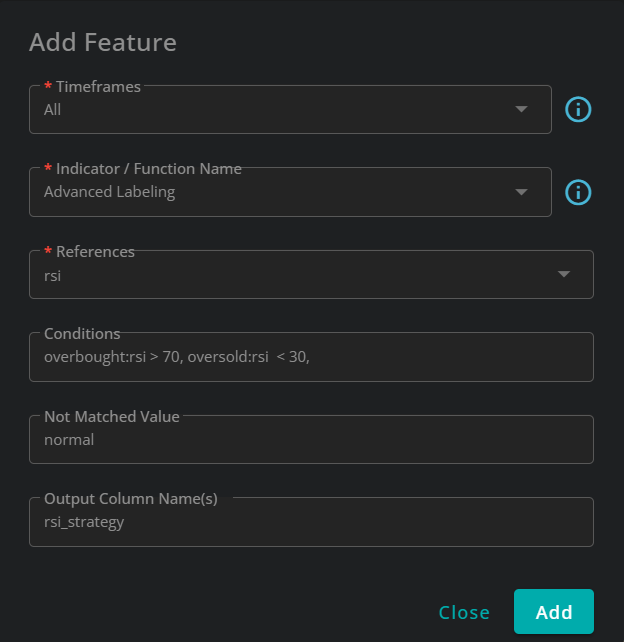
Use Advanced Labeling function to label candles as overbought, oversold and normal.
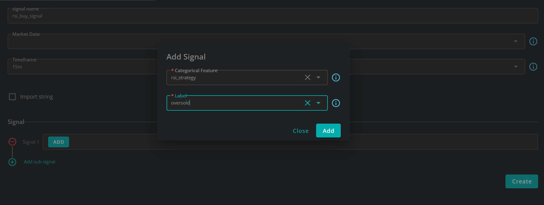
Use Signal Maker to make rsi_buy_signal and rsi_sell_signal signals that represent buying and selling signals of RSI.
The figures below illustrate how to use Advanced Labeling and Signal Maker to implement these signals.
For a detailed guide on using Advanced Labeling and Signal Maker, refer to the Beginner Series tutorial.


Stochastic Signals
Stochastic is a widely used technical indicator consisting of two lines: K and D. Similar to RSI, Stochastic identifies overbought and oversold regions:
Overbought: When K > 80, Stochastic suggests the market may be overbought.
Oversold: When K < 20, Stochastic suggests the market may be oversold.
However, Stochastic provides more precise signals through crossovers:
Buy Signal: When Stochastic is oversold (K < 20) and K crosses above D, it suggests a buy opportunity.
Sell Signal: When Stochastic is overbought (K > 80) and K crosses below D, it signals a sell opportunity.
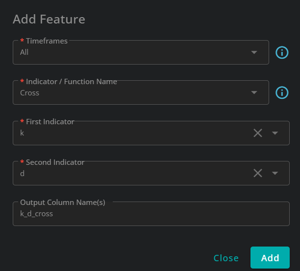
Use Cross function to detect:
Crossovers (when K moves above D) → potential buy signal.
Cross-unders (when K moves below D) → potential sell signal.
Use the same approach as RSI to classify candles as overbought and oversold.
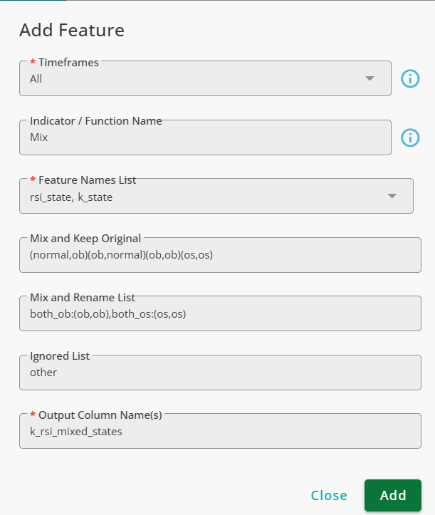
Use Mix function to define cross_over_over_sold and cross_under_over_bought labels.
Use Signal Maker once again to turn the last two labels to stoch_buy_signal and stoch_sell_signal.
The figures below demonstrate how to use Cross and Mix functions to implement these signals. For more details, refer to the Beginner Series tutorials and documentation.


Now that we have defined two buying and two selling signals, we can use Signal Analysis to assess their effectiveness.
How to use Signal Analysis
Signal Analysis provides various analytical tools, which we will explore in this tutorial. However, before using any of these tools, you need to configure the following settings:
Signal: Select the signal you want to analyze. You can choose any of the four signals we created in this tutorial.
Market Data: Choose the market data that contains the signals.
Pair(s): Select the pair(s) to include in the analysis. Note that to obtain accurate results, you must include a sufficient amount of data. In this tutorial, we use all three assets (Apple, Microsoft, and NVidia).
Timeframe: Select the timeframe for the analysis in. In this tutorial, we use a 15-minute timeframe.
Start Date: The first day of the analysis period.
End Date: The last day of the analysis period.
Numerical Target Analysis (NTA)
Numerical target Analysis evaluates the performance of your signals using a numeric target. A numeric target is any target with continuous values rather than discrete labels.
Any numeric target in QuantiX, including Rally-based Rating, Positive Momentum, etc. is compatible with NTA.
To use NTA:
select Numerical Target Analysis:
In the Report section, choose Numerical Target Analysis.
Choose a Reference Target:
Select the numeric target you want to analyze your signal against.
You can use:
Targets already added to your dataset.
A new target, which can be defined inline.
Finally, click on Get Report and wait for the system to process the data and display the results.
Signal Distribution
The Signal Distribution graph visualizes how frequently a signal was triggered across different ranges of the selected target.
The figure below illustrates Signal Distribution graph:
X-axis: Represents the ranges of the numeric target.
Y-axis: Displays the number of times the signal was triggered within each target range.
For this analysis, we used:
Target: Rally-Based Rating
Window Size: 100
Assets: Apple & Microsoft.
Timeframe: 15-minute
Report Period: 2021/01/01 – 2022/01/01
.png)
Numerical Target Analysis Summary
The Numerical Target Analysis Summary provides statistical insights into the distribution of signals over the selected numeric target, as visualized in the Signal Distribution graph.
The table includes the following metrics:
Mean, Median, STD, Minimum, and Maximum
The table below presents the summary statistics for the Signal Distribution graph shown earlier.

Numerical Target Analysis-Decomposition Analysis
If a signal consists of multiple sub-signals, the Decomposition Analysis breaks it down into its individual components. This allows for a more detailed evaluation of each sub-signal's performance.

Categorical Target Analysis (CTA)
Categorical Target Analysis evaluates the performance of a signal using a categorical target. Unlike numerical targets, categorical targets assign labels to candles, typically indicating buy, sell, or no-action signals.
Categorical targets supports various classification methods, including:
Rally-Based Classifying
Reward/Risk-Based Classifying
Positive Momentum Classifying
To use this tool:
In the Report section, choose Categorical Target Analysis.
Select the categorical target for the analysis. You can use:
A previously added target from your dataset.
A new target, which can be defined inline.
Finally, Click Get Report and wait for the system to process the data.
Precision Recall Summary
The Precision-Recall Summary chart provides a visual representation of the precision and recall for each target class.

Categorical Target Analysis Summary
The Summary Table reports the precision and recall of the signal for each class. This table presents the same values shown in the Precision-Recall Summary Chart in a structured format.
Additionally, it displays the number of times the signal was triggered for each class.

Decomposition Analysis
If a signal consists of multiple sub-signals, the Decomposition Analysis breaks it down into its components and provides the Summary Report for each sub-signal separately.

Rally Based Analysis
Rally-Based Analysis integrates the concept of rallies with precision and recall. Instead of counting individual signal occurrences, it groups price movements into rallies using a window size and then measures categorical target statistics for these rallies.
How Is Rally-Based Analysis Different from Categorical Target Analysis?
In Categorical Target Analysis, signals are counted each time they occur for a target label, meaning a signal may be counted multiple times within the same trend.
In Rally-Based Analysis, a signal is counted only once per rally, regardless of how many times it occurs within that rally.
To use this analysis:
Set a window size to define rallies.
The reports and tables generated follow the same format as those in Categorical Target Analysis.
The window size used for detecting rallies is independent of the settings used for the target in the analysis.
Stop Take Optimizer
This tool helps select stop-loss and take-profit levels for a signal. The evaluation metric used is the profit generated by the strategy under different stop-loss and take-profit settings.
The following configurations must be set:
Forward-Looking Window Length: The Stop-Take Optimizer evaluates how stop-loss and take-profit levels impact a signal’s performance by analyzing future data.
This setting determines the number of future candles used for each signal.
A longer window gives more time for stop-loss or take-profit conditions to be met.
If neither stop-loss nor take-profit is triggered within the window, the system closes the position at the end of the window and calculates the profit or loss.
Maximum Allowed Number of Signals per Window: A signal may be triggered multiple times within the forward-looking window.
Example:
If the window length is 100 candles and a second signal occurs 20 candles after the first, there will be two signals in the window.
If the maximum allowed number of signals per window is set to 1, the second signal is ignored, and only the first signal affects the profit/loss calculation.
If this value is set to greater than 1, the second signal is included in the analysis.
Maximum Stop Loss: The maximum value tested as stop-loss.
Maximum Take Profit: The maximum value tested as take-profit.
Stop Loss Resolution: This parameter determines the interval size between consecutive stop-loss values tested in the optimization process.
The Stop-Take Optimizer evaluates strategy performance for different stop-loss levels, ranging from 0 to the Maximum Stop Loss value.
Smaller resolution values result in more intervals, providing a higher resolution and more precise stop-loss optimization.
Take Profit Resolution: This parameter defines the interval size between consecutive take-profit values tested in the optimization process, ranging from 0 to the Maximum Take Profit value. The process works the same way as Stop Loss Resolution.
Fee (%): The fee represents the cost of trading, expressed as a percentage of each position. If a position is closed in loss, the fee of the position will be added to the loss.
Trading Side: This parameter specifies whether the signal is being used for long or short trading.
In this tutorial, we use Microsoft's market data from the first quarter of 2021 to determine the optimal stop-loss and take-profit values for the rsi_buy_strategy signal.
The settings of the analysis are as follows:
Forward-Looking Window Length: 100
Maximum Allowed Number of Signals per Window: 100
Maximum Stop Loss: 10
Maximum Take Profit: 10
Stop Loss Resolution: 1
Take Profit Resolution: 1
Fee (%): 0
Trading Side: Long
Profit Report
The Profit Report is a heatmap that visualizes the profitability of the signal across different stop-loss and take-profit values within the analysis period.
.png)
As seen in the heatmap, using take profits around 3% and stop losses less than 1% works best for this signal during the test range.
Win Rate Report
This report illustrates the win rate of the strategy for different stop loss and take profit intervals.
The win rate is calculated as:
Stop-loss > 1%
Take-profit < 1%
However, a higher win rate does not always mean higher profitability. For example, consider two strategies:
Strategy A: Opens one trade and closes it at 2% profit → Win rate: 100%
Strategy B: Opens five trades:
Three trades close at 5% profit each
Two trades close at 1% loss each
Win rate: 60%, but total profit = (3 × 5%) - (2 × 1%) = 13%, which is much higher than Strategy A.
.png)