QuantiX Indicators

QuantiX KAMA

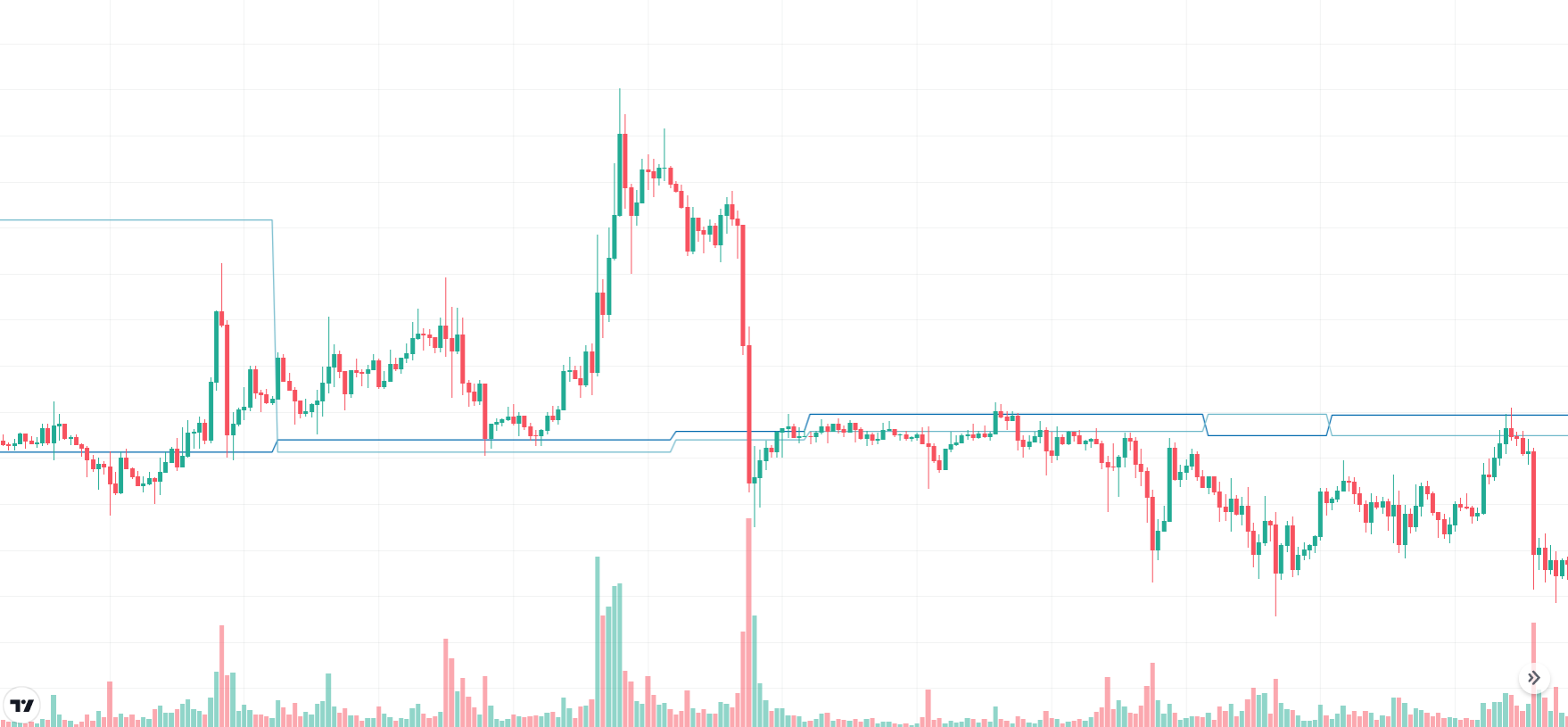
The QuantiX KAMA is an adaptive moving average designed to better follow price volatility while retaining a strong memory of past data. One common drawback of Simple Moving Averages (SMA) and Exponential Moving Averages (EMA) is the trade-off between responsiveness and memory—faster-moving averages lose historical context, while slower ones lag behind market movements. KiMA solves this issue by dynamically adjusting its window size based on historical market cycles, offering improved trend detection and acting as a robust support/resistance level.

This indicator is inspired by the studies of John Ehlers, a renowned mathematician, and adapts his concepts to optimize moving average performance.

QuantiX Fibonacci Retracement

The QuantiX Fibonacci Retracement function calculates Fibonacci retracement levels by identifying key pivot points in price action. This function returns three sets of lines:

• Last pivots: top and bottom

• Uptrend levels: fibut236, fibut382, fibut500, fibut618, and fibut786

• Downtrend levels: fibdt236, fibdt382, fibdt500, fibdt618, and fibdt786

The function utilizes the Pivot function to detect price pivots, generating Fibonacci retracement levels for both uptrends and downtrends:

• Uptrend retracement levels (fibut236 to fibut786) indicate potential resistance areas after a downtrend.

• Downtrend retracement levels (fibdt236 to fibdt786) indicate potential support areas after an uptrend.

• Top and Bottom store the latest high and low pivots, respectively.

When the most recent pivot is a low, use the uptrend retracement levels.
When the most recent pivot is a high, use the downtrend retracement levels.

Example

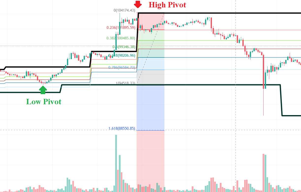
The default settings are used to find Fibonacci retracement levels. In the figure below, the thick black lines are the top and the button. As is seen, they match the last high and low pivot, respectively. The colored lines are downtrend levels calculated by the function, and the colorful region is Fibonacci retracement levels drawn by the Fib Retracement tool in tradingview. As is seen, they match each other.

QuantiX Fibonacci Expansion

This Fibonacci expansion implementation generates support and resistance levels. It returns two sets of outputs:

• Uptrend Levels: fibxut236, fibxut500, fibxut786, fibxut1000, fibxut1618

• Downtrend Levels: fibxdt236, fibxdt500, fibxdt786, fibxdt1000, fibxdt1618

Uptrend levels act as potential resistance points during an uptrend, while downtrend levels serve as potential support points during a downtrend. These levels are derived from previous pivots:

• Downtrend levels are calculated using two low pivots and one high pivot.

• Uptrend levels are calculated using two high pivots and one low pivot.

GCP

Green Candle Power (GCP) is an indicator developed by QuantiX team based on two concepts called Bull Power and Bear Power. For a green candle, bull and bear powers are calculated as follows:

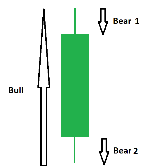
Bull power = (High - Low )

Bear power = (Bear 1 + Bear 2)

where :

Brear 1 = 100 * ((Open - Low) / Open)

Brear 2 = 100 * ((High - Close) / Open)

For a red candle the equations are as follows:

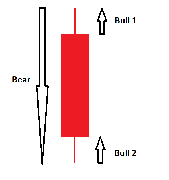
Bear Power = (High - Low )

Bull Power= (Bull 1 + Bull 2)

where :

Bull 1 = 100 * ((Close - Low) / Open)

Bull 2 = 100 * ((High - Open) / Open)

To mitigate the high volatility of Bull and Bear powers, moving averages of length Time Period is applied. and the output of this indicator will be three columns namely bear_rate, bull_rate, and gcp_rate. These values are:

bear_rate = SMA(Bear Power)

bull_rate = SMA(Bull Power)

gcp_rate = bull_rate - bear_rate

Use this indicator in the same manner that MACD is used. When gcp_rate becomes green, it is a possible sign of an upward rally, and when it becomes red, the market could be on the edge of a downward rally.

Example

Using the function's default settings, bull_rate, bear_rate, and gcp_rate are calculated and illustrated on the chart below.

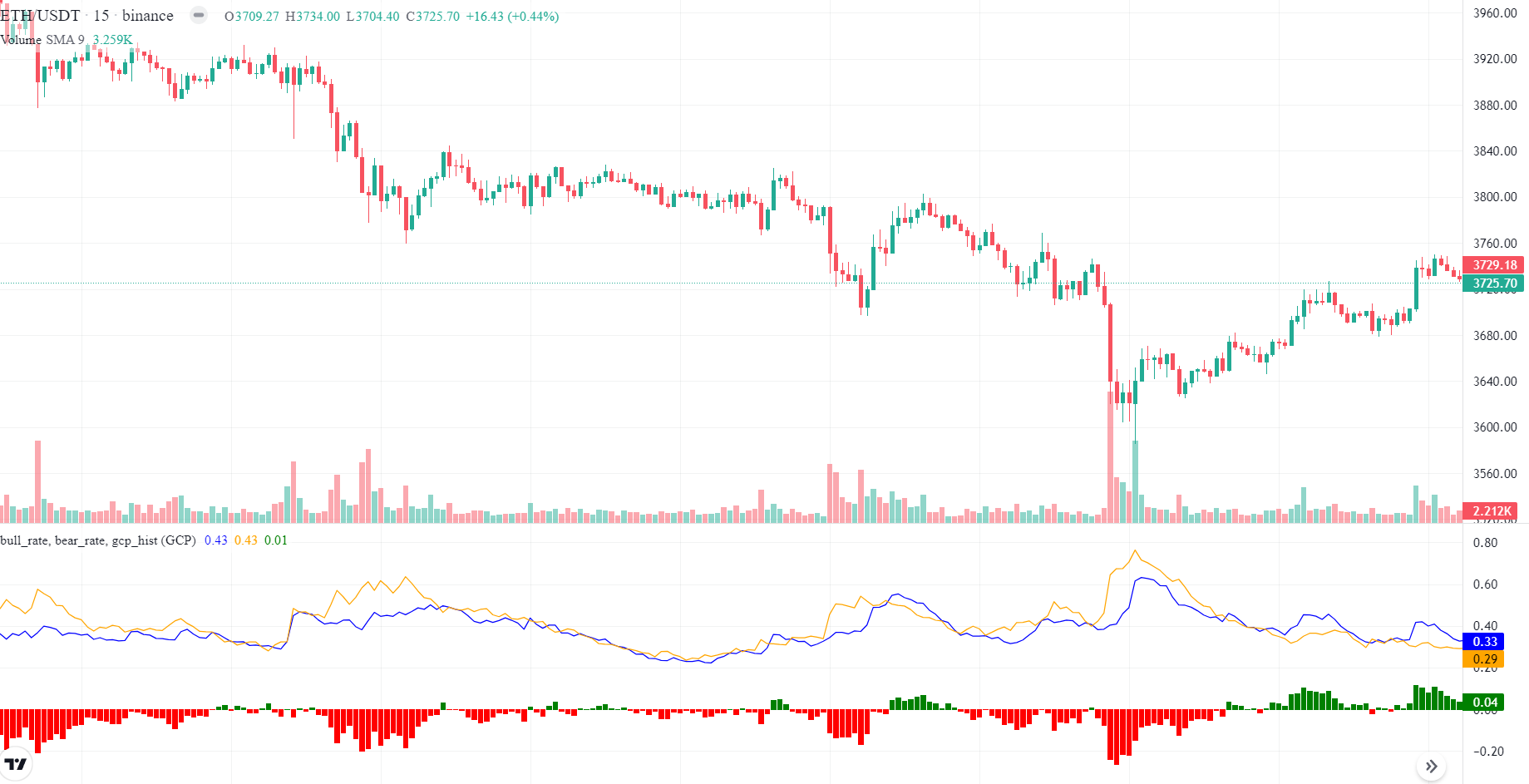
As is seen, the indicator behavior is close to MACD, with negative histogram values showing the domination of bears and positive values indicating the domination of bulls. Note that when histogram values become large, a trend direction change might be imminent.

Level

The level is an indicator exclusively available on QuantiX's platform and its goal is to help analysts better predict potential turning points (upcoming high pivots or low pivots). What this indicator is essentially doing is to make use of the previous pivots that lie within a window. This function aggregates the previous pivots' information that is within a user-defined range of the current price and returns a scalar that ranges between zero and one. The bigger this number is, the more previous pivots occurred around the current price. The following are the inputs of this indicator:

• Timeframes: the timeframes for which the indicator is calculated

• Pivot Window Length(s): the window length (s) used for pivot detection. ( For further details, please read the pivot function documentation)

• Sigma: Controls the pivot's magnitude of the effect; smaller values lead to pivots only affecting small neighborhoods around them and larger values dedicate larger spans to pivots. Using very small values will cause the indicator to become spiky and abrupt while very large sigmas leads to falsely high indicator values at unimportant prices.

• Pivot Weights: Controls the amount of influence the pivots of different window sizes have; the larger the corresponding weight of a window length becomes, the more influential its pivots will be in the final results.

• Pivot Types: Control the type of pivots (high pivots, low pivots,or both) considered in the calculations

• Look Backs: The size of the windows used to limit the previous pivots; note that for each pivot period, a different look back is defined.

• Interval Percent: The percentage of deviation from the price level to consider; e.g. for an interval percentage of 20, only pivot points that occurred within a price range of +/- 20% of the current price are accounted for.

• Interval Point Number: Controls the number of intervals that the range defined by Interval Percent is broken into

• Weights: Used to weight pivots with respect to another technical indicator; for example if the user sets Weights to volume , then pivots with larger volumes will have more effect in the final results.

• Fading Method: Recent pivots have more weight than older pivots; this parameter uses a specified method to assign less weight to older pivots. The basic setting is linear, which linearly increases the weight as it considers more recent candles.

• Projector Function: Controls the type of distribution function used to project previous pivots to the current candle on the horizontal axis ( i.e. price axis). Sigma is an internal parameter of this function.

• Column Name: the name of the column in which the result is stored.

Mean reversion

The Mean Reversion function models the mean reversion theory, allowing you to analyze the price's tendency to revert to a selected moving average. The function's output values can be either positive or negative—positive values indicate that the price is above the moving average, while negative values indicate that it is below.

To improve interpretability, the outputs are normalized using ATR (Average True Range). Assuming mean reversion holds true (though it remains an arguable conjecture rather than a proven theory), candles with significantly negative values in the output column may indicate strong buying opportunities, while highly positive values could suggest potential selling opportunities.

Inputs of this function are explained below.

Example

To model mean-reverting behavior of the market for a simple moving average with a window size of 30, we use Mean Reversion with the following configurations:

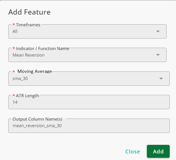
Note that you should add sma_30 (by using SMA function) first.

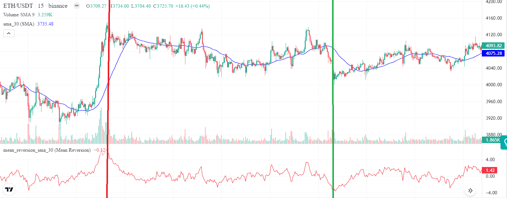
Using the Chart tool, you can see that when mean_reversion_sma_30 are large negative values, the price tends to go up (green line) and when they are large positive values (red line) the price tends to go down.

NMP V1 / NMP V2

Normalized Mean Profit (NMP) is a concept developed by the QuantiX team to model mean reversion in markets. Based on NMP, our team has created two indicators: NMP V1 and NMP V2. While both share a similar foundation, their modeling approaches differ.

You can use NMP V1 and NMP V2 similarly to the Relative Strength Index (RSI), as they feature overbought, oversold, and normal regions.

• For NMP V1, the overbought region includes values of +10 and above, while the oversold region consists of -10 and below.

• For NMP V2, the overbought threshold is 0.5, and the oversold threshold is -0.5.

The inputs of these functions are in the table below.

Example

To use NMP V1, we use the following settings:

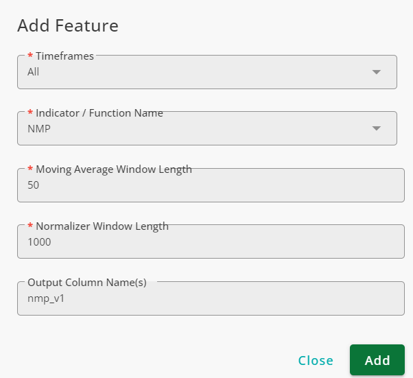
The result is shown in the figure below:

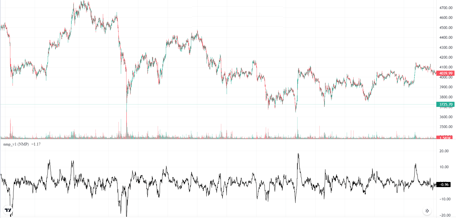
As is seen, the behavior of the indicator is similar to that of RSI.

Support Resistance

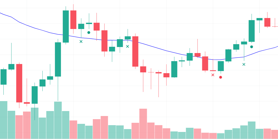
The Support Resistance function analyzes the close price against a specified level and determines whether the price reacts to that level. Candles are categorized as Other, Unconfirmed Support, Confirmed Support, Unconfirmed Resistance, or Confirmed Resistance.

• Unconfirmed Support: If the high price of a candle drops below the level but closes above it, the level is considered an unconfirmed support.

• Confirmed Support: If the next candle after an unconfirmed support remains entirely above the level (both body and shadows), it is confirmed as support.

• Unconfirmed Resistance: If the high price of a candle rises above the level but closes below it, the level is considered an unconfirmed resistance.

• Confirmed Resistance: If the next candle after an unconfirmed resistance remains entirely below the level (both body and shadows), it is confirmed as resistance.

Below is the list of the function's inputs.

Example

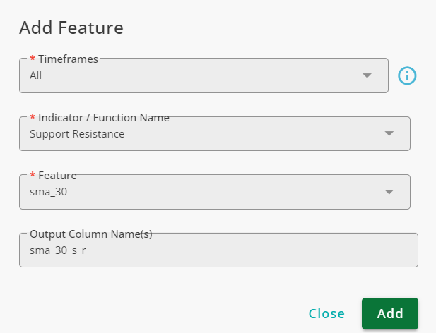
To check whether sma 30 acts as a support or resistance, you can use the Support Resistance function as is shown in the figure below:

In the figure below, confirmed supports and resistances are marked by green and red circles, respectively. Likewise, unconfirmed supports and resistances are marked by green and red crosses, respectively.

Previous Pivots

The Previous Pivots function propagates an arbitrary number of past pivots into the future. The primary purpose of this function is to allow users to incorporate the prices of previous pivots into their analysis.

The inputs of this function listed in the table below.

Example

Using the Previous Pivots function with the following configurations, we obtain the last four pivots ( four high and four low pivots).

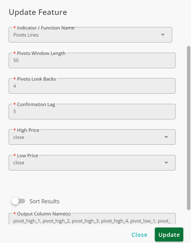
As is seen, for each candle, eight values corresponding to four high and four low pivots are returned.

Most Traded Price (MTP)

The Most Traded Price (MTP) uses the candle volumes in rallies to find important price levels. The indicator's logic says the price levels with higher volumes (and more trades as a result) are important, and the price reacts when it hits these levels. MTP returns the two most recent levels in its outputs.

The inputs of this indicator are listed below.

Example

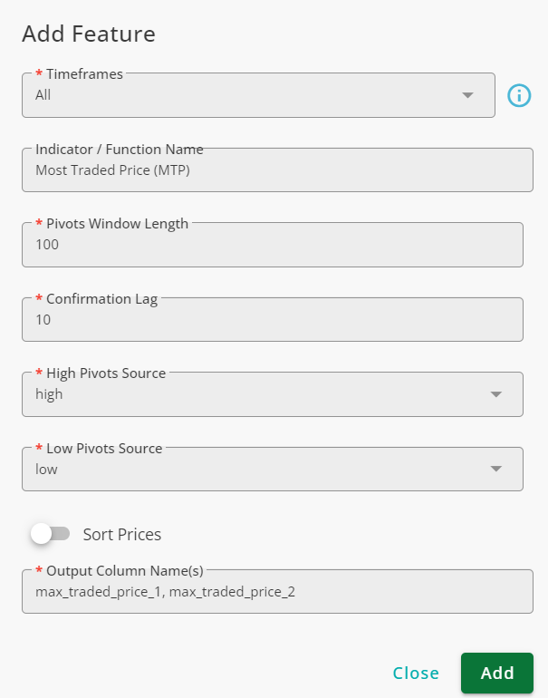
Using MTP with the following settings, we obtain two most traded price levels.

As is seen, the price reacts when it meets most traded price levels. In other words, these levels behave like support/resistance levels and are potent to change the direction of the price.